# show graphs in the notebooks and some config to make to look better

from matplotlib import pyplot as plt
plt.rcParams['figure.figsize'] = (8,4)
plt.style.use('ggplot')

%matplotlib inline2 Introduction to Data Analysis and Visualization
Python provides very intutive and powerful tools for data analysis. In this lesson, we’ll learn the concepts and see how to apply those to get insights from the data.
2.1 Numpy
Numpy is the numerical computation library in Python and this is the basis for most scientific computing and data science tools in Python. It is not only a building block, but many of these tools inherit the API of numpy for vector operatons and data selection. Understanding numpy closely helps us to use those tools better.
While you may not deal with numpy array directly, this knowledge will be useful in working with most data analysis tools in Python.
In this section, we’ll learn about the following things about numpy arrays:
- creation of multi-dimentional arrays
- reshaping them
- vector operations
- indexing
import numpy as npNumpy is a libray that provide a multi-dimentional array interface, with very elegant API.
Let’s start with creating a simple 1-dimentional array. Unlike lists in Python, all the elements of a numpy array will be of the same type.
x = np.array([1, 2, 3, 4, 5])xarray([1, 2, 3, 4, 5])x.shape(5,)x.dtypedtype('int64')Every array in numpy has a dtype and a shape. The dtype indicates the datatype of each element in the array and shape indicates the length of the array in each dimension as a tuple.
x = np.array([0.1, 0.2, 0.3])x.dtypedtype('float64')# create a float64 array with given numbers
x = np.array([1, 2, 3, 4], dtype=np.float64)xarray([1., 2., 3., 4.])x.dtypedtype('float64')We can create a two dimentional array as well.
d = np.array([
    [1, 2, 3],
[4, 5, 6]])darray([[1, 2, 3],
[4, 5, 6]])d.shape(2, 3)d.dtypedtype('int64')2.1.1 Utilties foc creating arrays
Numpy provides some utilities for creating arrays.
Create an array of zeros.
np.zeros(4)array([0., 0., 0., 0.])np.zeros((2, 4))array([[0., 0., 0., 0.],
[0., 0., 0., 0.]])# create a 1-d array of size 6 and reshape it 2-d array of size 2x3
np.zeros(6).reshape(2, 3)array([[0., 0., 0.],
[0., 0., 0.]])# create a 1-d array of size 24 and reshape it 3-d array of size 2x3x4
np.zeros(24).reshape(2, 3, 4)array([[[0., 0., 0., 0.],
[0., 0., 0., 0.],
[0., 0., 0., 0.]],
[[0., 0., 0., 0.],
[0., 0., 0., 0.],
[0., 0., 0., 0.]]])You can also create an array of ones.
np.ones(10)array([1., 1., 1., 1., 1., 1., 1., 1., 1., 1.])x = np.ones(10)x.dtypedtype('float64')x = np.ones(10, dtype=np.int8)xarray([1, 1, 1, 1, 1, 1, 1, 1, 1, 1], dtype=int8)x.dtypedtype('int8')Or a range of numbers using np.arange which works like range, but returns a numpy array.
np.arange(6)array([0, 1, 2, 3, 4, 5])np.arange(1, 2, 0.1)array([1. , 1.1, 1.2, 1.3, 1.4, 1.5, 1.6, 1.7, 1.8, 1.9])np.arange(1, 2, 0.1).reshape(2, 5)array([[1. , 1.1, 1.2, 1.3, 1.4],
[1.5, 1.6, 1.7, 1.8, 1.9]])2.1.1.1 Problem: Create a 3-d numpy array
Create a numpy array of shape (5, 4, 3) with all zeros.
2.1.2 Vector operations
The most interesting part of numpy arrays is the vector operations.
x = np.arange(1, 5)xarray([1, 2, 3, 4])When we use arthemetic operations on numpy arrays, those operations work on each element.
x + 10array([11, 12, 13, 14])x * 2array([2, 4, 6, 8])# python lists work differently
[1, 2, 3, 4] * 2[1, 2, 3, 4, 1, 2, 3, 4]x * xarray([ 1, 4, 9, 16])x ** xarray([ 1, 4, 27, 256])2 * x / 3array([0.66666667, 1.33333333, 2. , 2.66666667])How to compute sum of squares of all numbers below one million?
x = np.arange(1000000)
np.sum(x*x)333332833333500000Numpy is high-performance. The core computation engine is written in C language.
%%timeit
x = np.arange(1000000)
np.sum(x*x)
3.95 ms ± 167 µs per loop (mean ± std. dev. of 7 runs, 100 loops each)Compare the same with the simple python implementation.
%%timeit
x = range(1000000)
sum([i * i for i in x])
115 ms ± 5.89 ms per loop (mean ± std. dev. of 7 runs, 10 loops each)Notice that numpy is about 30X faster than the pure python version in this case.
The `timeit` is a jupyterlab magic command to find the time taken to execute a block of code.

It executes the block of code multiple times and reports the mean time along with standard deviation across runs.
2.1.2.1 Example: Computing Euclidian Distance
Euclidian distance between two vectors is defines as:
\(E(p,q) = \sqrt{\Sigma_{i=1}^{n}{(p_{i}-q_{i})^2}}\)
Write a function euclidian_distance to compute the euclidian distance between two vectors specified as numpy arrays.
def euclidian_distance(p, q):
    d = p-q
    total = np.sum(d*d)
    return np.sqrt(total)
p = np.array([1.0, 2.0, 3.0])
q = np.array([4.0, 5.0, 6.0])np.sqrt(np.sum((p-q)**2))5.196152422706632euclidian_distance(p, q)5.196152422706632euclidian_distance(p, p)0.02.1.2.2 Problem: Manhattan Distance
Write a function manhattan_distance to compute the manhattan distance between two vectors.
The manhattan distance is defined as:
\(M(p,q) = \Sigma_{i=1}^{n}{|pi−qi|}\)
For more info see: https://en.wikipedia.org/wiki/Taxicab_geometry
>>> manhanttan_distance(np.array([0,0]), np.array([3, 4]))
7
Hint: See numpy.abs.
x = np.array([-1.0, 0.5, -0.5])xarray([-1. , 0.5, -0.5])np.abs(x)array([1. , 0.5, 0.5])def manhanttan_distance(p, q):
...p = np.array([0, 0, 0, 0])
q = np.array([1, -2, 3, 4])
manhanttan_distance(p, q) # 102.1.3 Indexing and Slicing
Numpy provides interesting ways to select individual elements and parts of the array to enable operations on a subset of an array.
In the following examples, we are going to use the variable x for 1-d array and variable d for a 2-d array.
x = np.arange(1, 5, 0.5, dtype=np.float64)xarray([1. , 1.5, 2. , 2.5, 3. , 3.5, 4. , 4.5])d = x.reshape(2, 4)darray([[1. , 1.5, 2. , 2.5],
[3. , 3.5, 4. , 4.5]])We can access elements from a 1-d array just like a list.
x[0]1.0x[1]1.5When dealing with multi-dimentional arrays, we can specify a value for each dimension.
darray([[1. , 1.5, 2. , 2.5],
[3. , 3.5, 4. , 4.5]])d[0, 0]1.0d[0, 1]1.5d[1, 3]4.5We can also slice numpy arrays.
xarray([1. , 1.5, 2. , 2.5, 3. , 3.5, 4. , 4.5])x[:4]array([1. , 1.5, 2. , 2.5])x[4:]array([3. , 3.5, 4. , 4.5])The same rule applies for multi-dimentional arrays too, just that we need to specify value for bith dimensions.
d = np.arange(0, 12, 0.5).reshape(4, 6)darray([[ 0. , 0.5, 1. , 1.5, 2. , 2.5],
[ 3. , 3.5, 4. , 4.5, 5. , 5.5],
[ 6. , 6.5, 7. , 7.5, 8. , 8.5],
[ 9. , 9.5, 10. , 10.5, 11. , 11.5]])# top left corner
d[:2, :3]array([[0. , 0.5, 1. ],
[3. , 3.5, 4. ]])# bottom right corner?
d[2:, 3:]array([[ 7.5, 8. , 8.5],
[10.5, 11. , 11.5]])# Row 0
d[0, :] array([0. , 0.5, 1. , 1.5, 2. , 2.5])# Row 0
d[0]array([0. , 0.5, 1. , 1.5, 2. , 2.5])# Column 0
d[:, 0]array([0., 3., 6., 9.])Another interesting feature of numpy is boolean indexing.
xarray([1. , 1.5, 2. , 2.5, 3. , 3.5, 4. , 4.5])x > 2array([False, False, False, True, True, True, True, True])When we evaluate a boolean expression on an array, it is also considered as a vector operation and we get an array back.
The interesting thing is we can use that to select only the elements where there is True in the index.
For example, the following expression returns all the elements which are greater than 2.
x[x > 2]array([2.5, 3. , 3.5, 4. , 4.5])We could also use this to make some operations on them. For example. we want to double all the numbers that are greater than 2.
x[x > 2] *= 2xarray([1. , 1.5, 2. , 5. , 6. , 7. , 8. , 9. ])It is too boring and confusing to understand indexing just by staring numbers. Let’s take an example of a gray-scale image and see how these operations impact it.
2.1.4 Example: Gray Scale Image
We’ll use a sample image from scipy.
We are going to use matplotlib to display the image
import matplotlib.pyplot as plt
import scipy
face = scipy.datasets.face(gray=True)facearray([[114, 130, 145, ..., 119, 129, 137],
[ 83, 104, 123, ..., 118, 134, 146],
[ 68, 88, 109, ..., 119, 134, 145],
...,
[ 98, 103, 116, ..., 144, 143, 143],
[ 94, 104, 120, ..., 143, 142, 142],
[ 94, 106, 119, ..., 142, 141, 140]], dtype=uint8)face.shape(768, 1024)The shape is approximately 800x1000. We’ll use these numbers as approximation to make our computaion easy.
# function to show an image using matplotlib
def show(img):
    plt.imshow(img, cmap=plt.cm.gray)
show(face)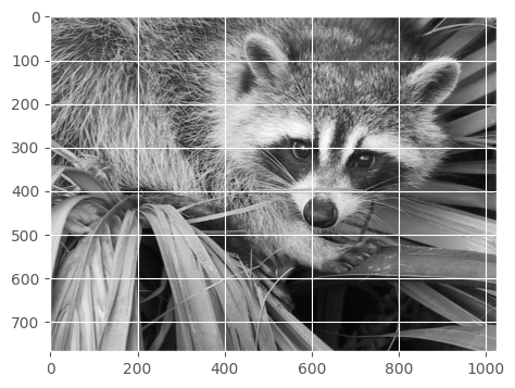
How to negate the image?
Each value in the array is between 0 to 255. What would we get if we try 255 - face?
show(255 - face)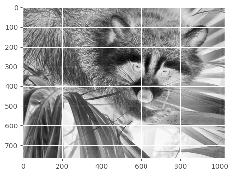
How to get the top-half of the face?
show(face[:400, :]) # a bit more than half, just lazy to compute height/2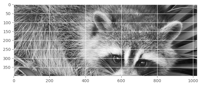
How to get the bottom half?
show(face[400:, :])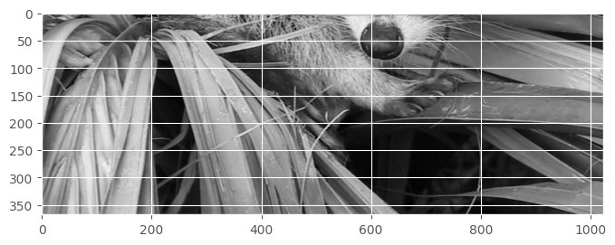
How to get the left half?
How to get the right half
Skip 100 pixels on all sides
show(face[100:-100, 100:-100])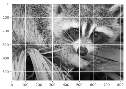
How to flip the image vertically?
show(face[:, ::-1])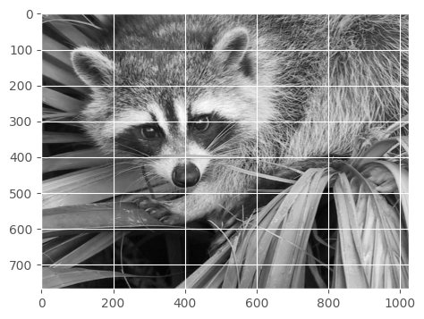
And flip horizontally…
show(face[::-1, :])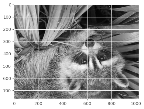
Add 10px border
We’ll just replace the 10 pixels on all sides with black.
face1 = face.copy() # make a copy because we are modifying itface1[:10, :] = 0
face1[-10:, :] = 0
face1[:, :10] = 0
face1[:, -10:] = 0show(face1)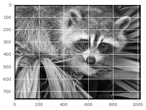
Can you try adding a 10px outer border with black color and another 10 px inner border with white color?
Make the image sharp
Turn all colors less than 200 to 0.
face1 = face.copy()face1[face1 < 200] = 0show(face1)2.2 Pandas
Pandas is library to work with tabular data in Python. In another words, Pandas is spereadsheet tool for hackers.
Pandas mainly has two classes Series and DataFrame. A DataFrame represents a tabular dataset and Series represents a column.
import pandas as pdLet’s start with a sample dataset.
df = pd.read_csv("shared/un-min.csv")Let’s see the first few rows of the dataframe.
df.head()| country | region | lifeMale | lifeFemale | infantMortality | GDPperCapita | |
|---|---|---|---|---|---|---|
| 0 | Afghanistan | Asia | 45.0 | 46.0 | 154 | 2848 |
| 1 | Albania | Europe | 68.0 | 74.0 | 32 | 863 |
| 2 | Algeria | Africa | 67.5 | 70.3 | 44 | 1531 |
| 3 | Angola | Africa | 44.9 | 48.1 | 124 | 355 |
| 4 | Argentina | America | 69.6 | 76.8 | 22 | 8055 |
len(df)188df.columnsIndex(['country', 'region', 'lifeMale', 'lifeFemale', 'infantMortality',
'GDPperCapita'],
dtype='object')df.dtypescountry object
region object
lifeMale float64
lifeFemale float64
infantMortality int64
GDPperCapita int64
dtype: objectPandas automatically infers the datatype when reading a csv file.
All the categorical columns with string values will be of type object.
df.describe()| lifeMale | lifeFemale | infantMortality | GDPperCapita | |
|---|---|---|---|---|
| count | 188.000000 | 188.000000 | 188.000000 | 188.000000 |
| mean | 63.526064 | 68.309043 | 44.308511 | 5890.595745 |
| std | 9.820235 | 11.085095 | 38.896964 | 8917.273130 |
| min | 36.000000 | 39.100000 | 3.000000 | 36.000000 |
| 25% | 57.275000 | 58.625000 | 12.000000 | 426.500000 |
| 50% | 66.500000 | 71.950000 | 30.500000 | 1654.500000 |
| 75% | 70.675000 | 76.250000 | 71.250000 | 6730.500000 |
| max | 77.400000 | 82.900000 | 169.000000 | 42416.000000 |
2.2.1 Accessing individual columns
Columns can be accessed using . or []. The . notation works only when the column name doesn’t have space or other special characters.
df.infantMortality0 154
1 32
2 44
3 124
4 22
...
183 37
184 80
185 19
186 103
187 68
Name: infantMortality, Length: 188, dtype: int64df["infantMortality"]The columns are like numpy arrays and we can do vector operations on them.
For example we can compute the avarage life expectency between male and female by taking average of them.
(df.lifeMale + df.lifeFemale)/20 45.50
1 71.00
2 68.90
3 46.50
4 73.20
...
183 67.25
184 57.90
185 72.55
186 42.95
187 48.50
Length: 188, dtype: float64How many regions are there?
df.region.head()0 Asia
1 Europe
2 Africa
3 Africa
4 America
Name: region, dtype: objectdf.region.unique()array(['Asia', 'Europe', 'Africa', 'America', 'Oceania'], dtype=object)df.region.nunique()5df.region.value_counts()Africa 53
Asia 46
Europe 40
America 35
Oceania 14
Name: region, dtype: int642.2.2 Index
Pandas supports having a row index and it is handy to keep an index when there is a column with unique name for each name.
df.set_index("country", inplace=True)df.head()| region | lifeMale | lifeFemale | infantMortality | GDPperCapita | |
|---|---|---|---|---|---|
| country | |||||
| Afghanistan | Asia | 45.0 | 46.0 | 154 | 2848 |
| Albania | Europe | 68.0 | 74.0 | 32 | 863 |
| Algeria | Africa | 67.5 | 70.3 | 44 | 1531 |
| Angola | Africa | 44.9 | 48.1 | 124 | 355 |
| Argentina | America | 69.6 | 76.8 | 22 | 8055 |
In most methods on dataframes return a new dataframe instead of modifying the same dataframe. Passing `inplace=True` changes that behavior to update the dataframe inplace.

Instead of using `inplace=True`, we could also do the following, but that would be more confusing.

    df = df.set_index("country")
We can reset the index by calling reset_index method. Again, we need to pass inplace=True if we want to modify the dataframe.
df.reset_index(inplace=True)df.head()Let’s put the index back the rest of our exploration.
df.set_index("country", inplace=True)df.head()We can access the index using df.index.
df.indexIndex(['Afghanistan', 'Albania', 'Algeria', 'Angola', 'Argentina', 'Armenia',
'Australia', 'Austria', 'Azerbaijan', 'Bahamas',
...
'United.States', 'Uruguay', 'Uzbekistan', 'Vanuatu', 'Venezuela',
'Viet.Nam', 'Yemen', 'Yugoslavia', 'Zambia', 'Zimbabwe'],
dtype='object', name='country', length=188)df.index[:5]Index(['Afghanistan', 'Albania', 'Algeria', 'Angola', 'Argentina'], dtype='object', name='country')2.2.3 Visualization
“A picture is worth a thousand words”
How is the wealth distributed across the world?
df.hist("GDPperCapita")array([[<Axes: title={'center': 'GDPperCapita'}>]], dtype=object)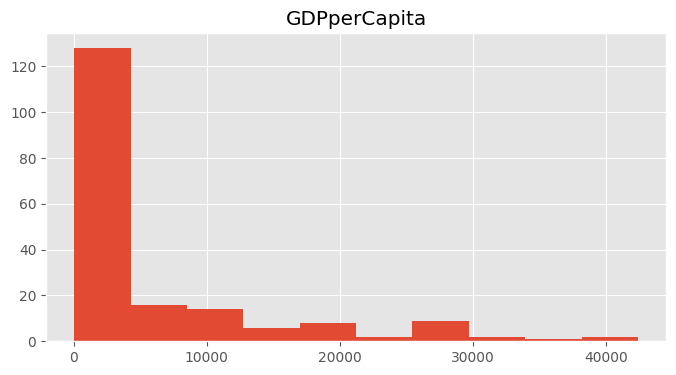
# we can also call histogram on the column
df.GDPperCapita.hist()df.boxplot("GDPperCapita")<Axes: >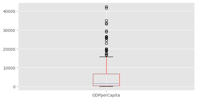
Does wealth corelate with health?
df.plot(kind="scatter", x="GDPperCapita", y="infantMortality")<Axes: xlabel='GDPperCapita', ylabel='infantMortality'>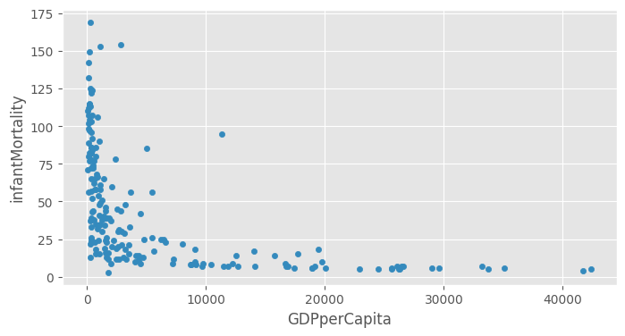
2.2.3.1 Problem: Plot lifeMale vs. lifeFemale
2.2.4 Sorting values
Lot of times we want to order data based on a column to see the top few values.
What are the top-10 rich countries.
df.sort_values("GDPperCapita")| region | lifeMale | lifeFemale | infantMortality | GDPperCapita | |
|---|---|---|---|---|---|
| country | |||||
| Sudan | Africa | 53.6 | 56.4 | 71 | 36 |
| Mozambique | Africa | 45.5 | 48.4 | 110 | 77 |
| Ethiopia | Africa | 48.4 | 51.6 | 107 | 96 |
| Eritrea | Africa | 49.1 | 52.1 | 98 | 96 |
| Dem.Rep.of.the.Congo | Africa | 51.3 | 54.5 | 89 | 117 |
| ... | ... | ... | ... | ... | ... |
| Denmark | Europe | 73.0 | 78.3 | 7 | 33191 |
| Norway | Europe | 74.8 | 80.6 | 5 | 33734 |
| Luxembourg | Europe | 73.1 | 79.7 | 6 | 35109 |
| Japan | Asia | 76.9 | 82.9 | 4 | 41718 |
| Switzerland | Europe | 75.3 | 81.8 | 5 | 42416 |
188 rows × 5 columns
df.sort_values("GDPperCapita", ascending=False).head()| region | lifeMale | lifeFemale | infantMortality | GDPperCapita | |
|---|---|---|---|---|---|
| country | |||||
| Switzerland | Europe | 75.3 | 81.8 | 5 | 42416 |
| Japan | Asia | 76.9 | 82.9 | 4 | 41718 |
| Luxembourg | Europe | 73.1 | 79.7 | 6 | 35109 |
| Norway | Europe | 74.8 | 80.6 | 5 | 33734 |
| Denmark | Europe | 73.0 | 78.3 | 7 | 33191 |
df.sort_values("GDPperCapita", ascending=False).head().indexIndex(['Switzerland', 'Japan', 'Luxembourg', 'Norway', 'Denmark'], dtype='object', name='country')(df.GDPperCapita
.sort_values(ascending=False)
.head(20)
.plot(kind="bar"))<Axes: xlabel='country'>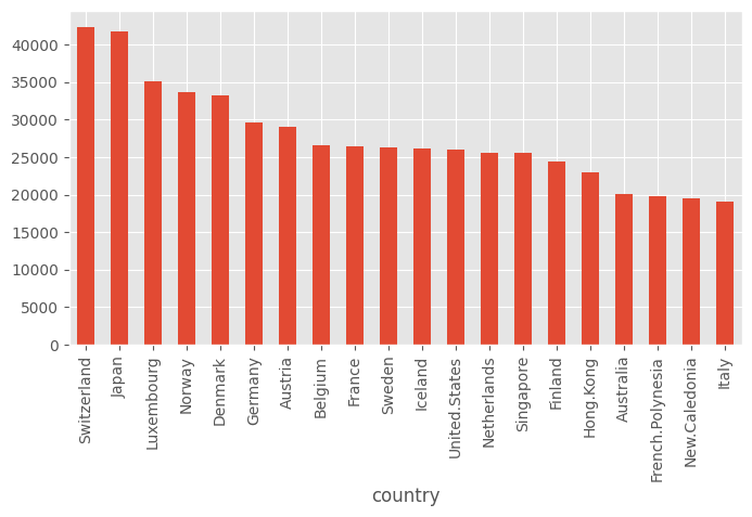
2.2.4.1 Problem: What are the 10 poorest countries?
2.2.4.2 Problem: What are the 10 counties with really bad infantMortality?
2.2.5 Group By
Group By is a powerful tool to summarize values on a column.
In this example we have data by country, what if we want to summarize the data by the region?
df.head()| region | lifeMale | lifeFemale | infantMortality | GDPperCapita | |
|---|---|---|---|---|---|
| country | |||||
| Afghanistan | Asia | 45.0 | 46.0 | 154 | 2848 |
| Albania | Europe | 68.0 | 74.0 | 32 | 863 |
| Algeria | Africa | 67.5 | 70.3 | 44 | 1531 |
| Angola | Africa | 44.9 | 48.1 | 124 | 355 |
| Argentina | America | 69.6 | 76.8 | 22 | 8055 |
df.groupby("region").mean()| lifeMale | lifeFemale | infantMortality | GDPperCapita | |
|---|---|---|---|---|
| region | ||||
| Africa | 52.052830 | 55.286792 | 86.320755 | 1217.641509 |
| America | 69.082857 | 74.474286 | 26.657143 | 5080.085714 |
| Asia | 65.373913 | 69.439130 | 43.782609 | 5453.195652 |
| Europe | 70.362500 | 77.545000 | 11.575000 | 12860.050000 |
| Oceania | 67.464286 | 72.092857 | 24.642857 | 7131.785714 |
Notice that the index has become the column on which we did group by. Also, all the categorical columns are ignored on group by.
df_region = df.groupby("region").mean()df_region.GDPperCapita.plot(kind="bar")<Axes: xlabel='region'>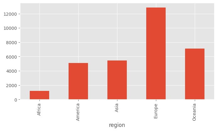
2.2.6 Selecting Rows
A lot of times, we want to work on a subset of the dataset to drill down for specific insights.
The vector operations that we learnt in numpy comes handy here.
df_africa = df[df.region == "Africa"]df_africa.head()| region | lifeMale | lifeFemale | infantMortality | GDPperCapita | |
|---|---|---|---|---|---|
| country | |||||
| Algeria | Africa | 67.5 | 70.3 | 44 | 1531 |
| Angola | Africa | 44.9 | 48.1 | 124 | 355 |
| Benin | Africa | 52.4 | 57.2 | 84 | 391 |
| Botswana | Africa | 48.9 | 51.7 | 56 | 3640 |
| Burkina.Faso | Africa | 45.1 | 47.0 | 97 | 165 |
df_africa.plot(kind="scatter", x="GDPperCapita", y="infantMortality")<Axes: xlabel='GDPperCapita', ylabel='infantMortality'>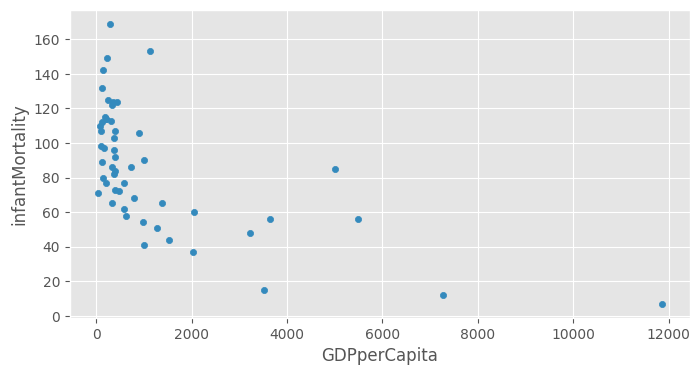
Let’s select poor countries.
df.GDPperCapita.hist()<Axes: >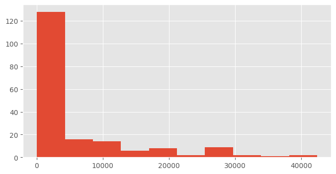
df_poor = df[df.GDPperCapita < 1000]df_poor.head()| region | lifeMale | lifeFemale | infantMortality | GDPperCapita | |
|---|---|---|---|---|---|
| country | |||||
| Albania | Europe | 68.0 | 74.0 | 32 | 863 |
| Angola | Africa | 44.9 | 48.1 | 124 | 355 |
| Armenia | Europe | 67.2 | 74.0 | 25 | 354 |
| Azerbaijan | Asia | 66.5 | 74.5 | 33 | 321 |
| Bangladesh | Asia | 58.1 | 58.2 | 78 | 280 |
len(df_poor)73len(df)188Which regions have more poor countries?
df_poor.region.value_counts()Africa 39
Asia 20
Europe 6
America 6
Oceania 2
Name: region, dtype: int642.2.6.1 Problem: Find the poor countries in Europe?
Find the countries in Europe that has GDPperCapita less than 1000.
df[(df.GDPperCapita < 1000) & (df.region == "Europe")]| region | lifeMale | lifeFemale | infantMortality | GDPperCapita | |
|---|---|---|---|---|---|
| country | |||||
| Albania | Europe | 68.0 | 74.0 | 32 | 863 |
| Armenia | Europe | 67.2 | 74.0 | 25 | 354 |
| Belarus | Europe | 64.4 | 74.8 | 15 | 994 |
| Bosnia | Europe | 70.5 | 75.9 | 13 | 271 |
| Moldova | Europe | 63.5 | 71.5 | 26 | 383 |
| Ukraine | Europe | 63.6 | 74.0 | 18 | 694 |
2.2.6.2 Drilling down Further
Let’s look at the wealth vs health graph again.
df.plot(kind="scatter", x="GDPperCapita", y="infantMortality")Which are the countries that are rich, but not doing well on health?
df[(df.GDPperCapita > 1000) & (df.infantMortality > 100)]| region | lifeMale | lifeFemale | infantMortality | GDPperCapita | |
|---|---|---|---|---|---|
| country | |||||
| Afghanistan | Asia | 45.0 | 46.0 | 154 | 2848 |
| Liberia | Africa | 50.0 | 53.0 | 153 | 1124 |
Which are the countries that are not that rich, but not well on health?
df[(df.GDPperCapita < 500) & (df.infantMortality < 50)]| region | lifeMale | lifeFemale | infantMortality | GDPperCapita | |
|---|---|---|---|---|---|
| country | |||||
| Armenia | Europe | 67.2 | 74.0 | 25 | 354 |
| Azerbaijan | Asia | 66.5 | 74.5 | 33 | 321 |
| Bosnia | Europe | 70.5 | 75.9 | 13 | 271 |
| Georgia | Asia | 68.5 | 76.7 | 23 | 343 |
| Korea.Dem.Peoples.Rep | Asia | 68.9 | 75.1 | 22 | 271 |
| Kyrgyzstan | Asia | 63.4 | 71.9 | 39 | 331 |
| Moldova | Europe | 63.5 | 71.5 | 26 | 383 |
| Nicaragua | America | 65.8 | 70.6 | 44 | 464 |
| Uzbekistan | Asia | 64.3 | 70.7 | 43 | 435 |
| Viet.Nam | Asia | 64.9 | 69.6 | 37 | 270 |
2.2.7 Problem: Find the countries which have large gap between lifeMale vs. lifeFemale
For reference look at the scatter plot of lifeMale vs. lifeFemale.
df.plot(kind="scatter", x="lifeMale", y="lifeFemale")df.plot?