5  Interfacing R from Python

While Python is quite versatile language that makes solving problems very simple, the language R has its own strengths. It has been very popular in the academic circles and many of the bioinformatics algorithms often gets released as R packages. Often, the only possible way solve a particular problem effectively is using R.

It is pragmatic to use the right tool for the right job. In this session, we’ll see how to use R from Python. We’ll see two different approaches - using R from jupyter notebooks along with Python and using R in scripts and streamlit applications.

5.1 The rpy2 package

The rpy2 package in Python provides a way to execute R from python and it also has good support for jupyter notebooks.

5.1.1 Using R in the notebook

Import rpy2 package.

import rpy2

And load rpy2 jupyter extension.

%load_ext rpy2.ipython

Now we can run R code and even plot graphs.

%%R 
library(palmerpenguins)

# Print the first 6 rows
head(penguins, 6)

plot(penguins$bill_length_mm, penguins$bill_depth_mm)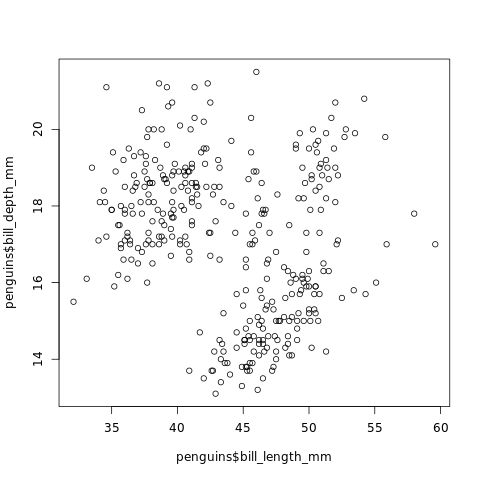

You can even use the familiar ggplot2 library.

%%R 

# Whatever we have run earlier in R will still be available here.

library(ggplot2)

ggplot(penguins, aes(bill_length_mm, bill_depth_mm, colour = species)) + 
  geom_point()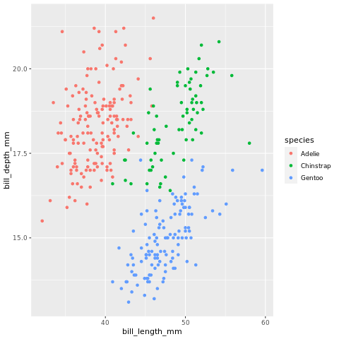

5.2 Passing values between Python and R

import pandas as pd

Define two of values in Python.

x = 10
y = 20

Add add them in R.

%%R -i x -i y

x + y

[1] 30

It is even possible to access the value of a variable define in R from Python, but we’ll look into into it later.

Interesting part of this approach is that we can even pass dataframes into R.

df = pd.read_csv("../shared/un-min.csv")

df.head()

	country	region	lifeMale	lifeFemale	infantMortality	GDPperCapita
0	Afghanistan	Asia	45.0	46.0	154	2848
1	Albania	Europe	68.0	74.0	32	863
2	Algeria	Africa	67.5	70.3	44	1531
3	Angola	Africa	44.9	48.1	124	355
4	Argentina	America	69.6	76.8	22	8055

%%R -i df

library(ggplot2)

ggplot(df, aes(GDPperCapita, infantMortality, colour = region)) + 
  geom_point()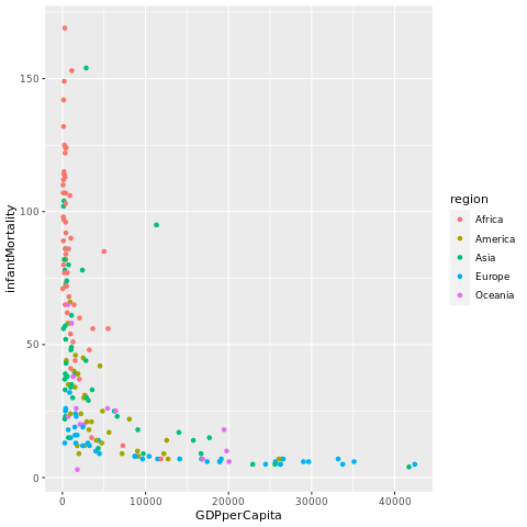

Question: Can we read dataframe in R and get it to Python and plot?

An easy way is to write the dataframe in R to a file and read it in python. We’ll look into another approach in a later section.

%%R

data(mtcars)
head(mtcars)

write.csv(mtcars, "mtcars.csv")

!ls -l mtcars.csv

-rw-r--r-- 1 anand anand 1783 Jun  3 03:59 mtcars.csv

df = pd.read_csv("mtcars.csv")

df.head()

	Unnamed: 0	mpg	cyl	disp	hp	drat	wt	qsec	vs	am	gear	carb
0	Mazda RX4	21.0	6	160.0	110	3.90	2.620	16.46	0	1	4	4
1	Mazda RX4 Wag	21.0	6	160.0	110	3.90	2.875	17.02	0	1	4	4
2	Datsun 710	22.8	4	108.0	93	3.85	2.320	18.61	1	1	4	1
3	Hornet 4 Drive	21.4	6	258.0	110	3.08	3.215	19.44	1	0	3	1
4	Hornet Sportabout	18.7	8	360.0	175	3.15	3.440	17.02	0	0	3	2

df.plot(kind="scatter", x="mpg", y="hp")

<Axes: xlabel='mpg', ylabel='hp'>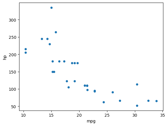

Problem: Plot a graph of lifeMale vs. lifeFemale, color by region and size by th GDP using ggplot2 in R.

Problem: Read iris dataset from ../shared/iris.csv in Python and plot a scatter plot on SepalLength vs. SepalWidth and color by Name using R.

5.3 Invoking R programatically

Invoking R programatically can be done using the rpy2 package without using the %%R magic method.

The rpy2 module allows passing inputs to R and read the results back. While there may be issues with convertion of types between python and R, it will be simpler if we stick to primitive and well known types.

To make things simple for you, I have created a function rexec.

import rpy2.robjects as robjects
from rpy2.robjects import pandas2ri
from rpy2.robjects.conversion import localconverter

def rexec(code, **params):
    """Script to run R code passing some inputs to it.

        >>> rexec("print(x+y)", x=10, y=20)
        [1] 30

    If you would like to get back some result from R, assign that 
    to variable result.

        >>> rexec("result <- x + y", x=10, y=20)
        array([30], dtype=int32)
    """
    # rpy2 has some multi-threading issues and this is the recommended way to convert python objects to R
    # See https://github.com/rpy2/rpy2/issues/978
    with localconverter(robjects.default_converter + pandas2ri.converter) as cv:
        robjects.globalenv['result'] = False
        for k, v in params.items():
            robjects.globalenv[k] = cv.py2rpy(v)
        robjects.r(code)

        result = robjects.r.get("result")
        if result is not None:
            return cv.rpy2py(result)

rexec("print(x+y)", x=10, y=20)

[1] 30

BoolVector with 1 elements.

0

z = rexec("result <- x+y", x=10, y=20)

z

array([30], dtype=int32)

z[0]

30

5.3.1 Ploting and Saving Graphs

Now, let us look at running a complete R script from python by passing inputs and outputs only through files.

It reads the input from ../shared/un-min.csv and write the graph as image to rplot.png.

df = pd.read_csv("../shared/un-min.csv")

df.head()

	country	region	lifeMale	lifeFemale	infantMortality	GDPperCapita
0	Afghanistan	Asia	45.0	46.0	154	2848
1	Albania	Europe	68.0	74.0	32	863
2	Algeria	Africa	67.5	70.3	44	1531
3	Angola	Africa	44.9	48.1	124	355
4	Argentina	America	69.6	76.8	22	8055

code = """
library(ggplot2)

ggplot(df, aes(GDPperCapita, lifeFemale, colour = region)) + 
  geom_point()
  
ggsave(filename = image_path) 
"""

rexec(code, df=df, image_path="rplot.png")

Saving 7 x 7 in image

BoolVector with 1 elements.

0

!ls -l *.png

-rw-r--r-- 1 anand anand 136075 Jun  3 04:13 rplot.png

from IPython.display import Image

Image(filename="rplot.png")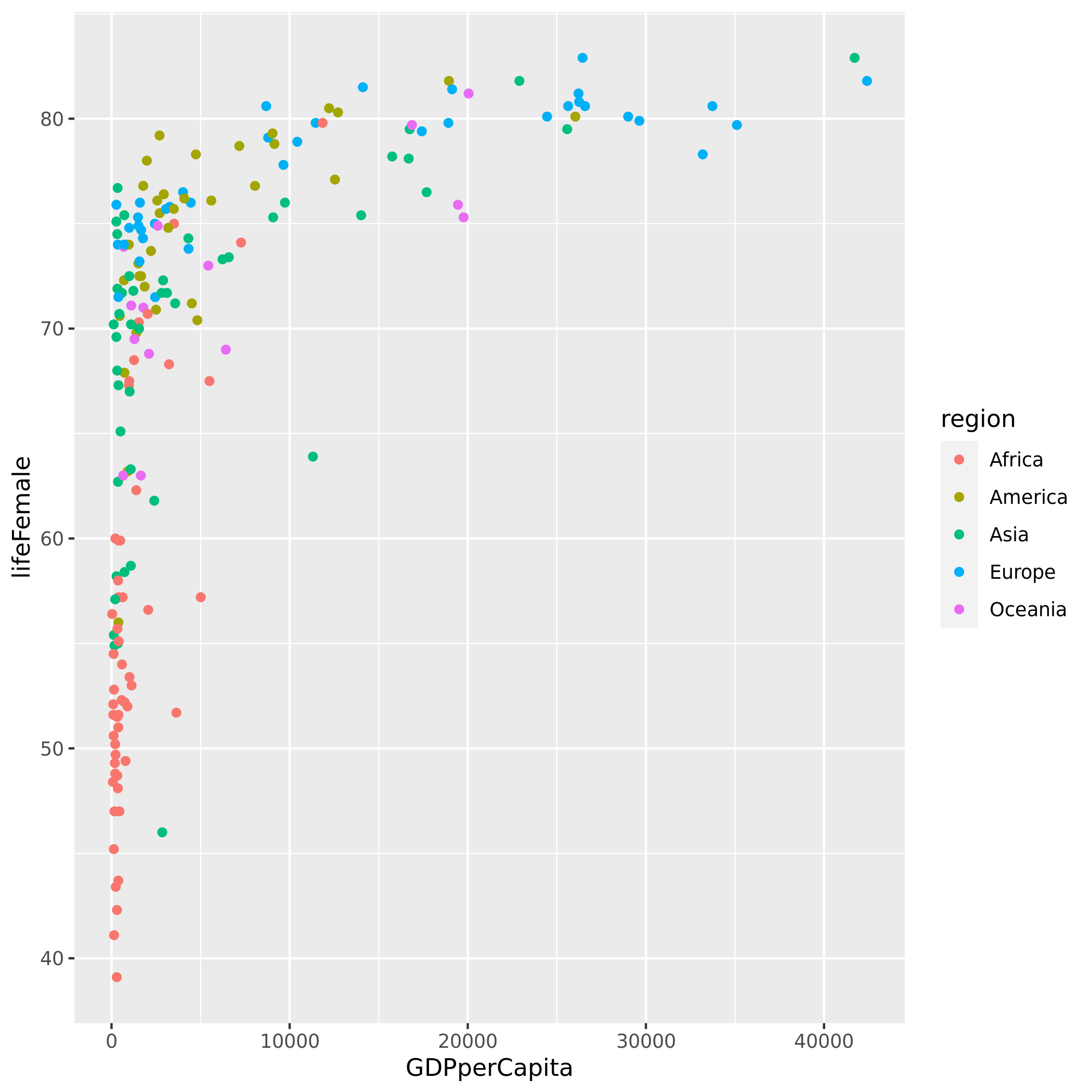

Q: Can we do some analysis in R and get the results back in Python for plotting?

Let’s take iris dataset, pass it to R for aggregation, get the result back to Python and plot them.

df.head()

	country	region	lifeMale	lifeFemale	infantMortality	GDPperCapita
0	Afghanistan	Asia	45.0	46.0	154	2848
1	Albania	Europe	68.0	74.0	32	863
2	Algeria	Africa	67.5	70.3	44	1531
3	Angola	Africa	44.9	48.1	124	355
4	Argentina	America	69.6	76.8	22	8055

df.set_index("country", inplace=True)

df.head()

	region	lifeMale	lifeFemale	infantMortality	GDPperCapita
country
Afghanistan	Asia	45.0	46.0	154	2848
Albania	Europe	68.0	74.0	32	863
Algeria	Africa	67.5	70.3	44	1531
Angola	Africa	44.9	48.1	124	355
Argentina	America	69.6	76.8	22	8055

code = """
df2 <- aggregate(. ~ region, df, mean)
result <- df2
"""

rexec(code, df=df)

	region	lifeMale	lifeFemale	infantMortality	GDPperCapita
1	Africa	52.052830	55.286792	86.320755	1217.641509
2	America	69.082857	74.474286	26.657143	5080.085714
3	Asia	65.373913	69.439130	43.782609	5453.195652
4	Europe	70.362500	77.545000	11.575000	12860.050000
5	Oceania	67.464286	72.092857	24.642857	7131.785714